Hide or Remove Grand Total in Pivot Table
When you create a Pivot Table, Microsoft Excel will automatically add a Grand Total Row, Grand Total column, depending on the organization of your Pivot Table. However, some reporting requirements may not actually need Grand Total Rows or Grand Total Columns. Hence, we are providing below the steps to hide Grand Total in Pivot Table rows or columns.
Steps to Remove Grand Total in Pivot Table
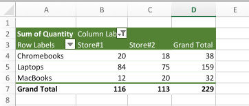
As you can see in the Pivot Table below, we have the “Subtotals” for products sold by Store#1 and Store#2 and also the “Grand Total” of all the Products sold by the two Stores.
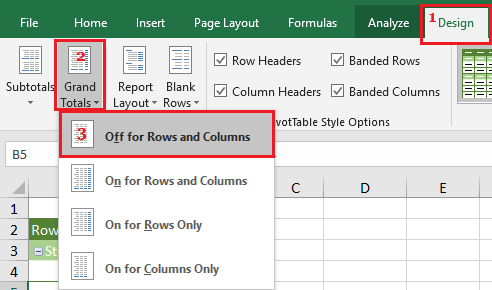
Since, we are only interested in tracking the individual sales made by the two stores, we are going ahead with the following steps to remove Grand Total in this pivot table. 1. Click on any Cell in the Pivot Table and you will see 2 new tabs (Analyze & Design) appearing on the top menu bar. 2. Next, click on the Design tab > click on Grand Totals and select OFF for Rows and Columns option in the drop-down menu.
This will totally remove Grand Totals from your Pivot Table and the Pivot Table will only indicate the subtotals.
Hide Column or Row Grand Totals in Pivot Table
As you can see in the image below, we have a Pivot Table showing both Row and Column grand totals. Since, this is not necessary in our case, we are going ahead with the following steps to remove Row Grand Totals in Pivot Table.
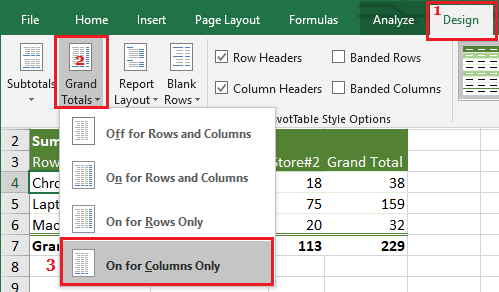
- Click on any Cell in the Pivot Table and you will see 2 new tabs (Analyze & Design) appearing on the top menu bar. 2. Click on the Design Tab > click on Grand Totals and select On for Columns Only option in the drop-down menu.
Now if you take a look at your worksheet, you will only see Column Grand Totals and Row Grand Totals will be removed in the Pivot Table.
How to Add or Remove Subtotals in Pivot Table How to Create Pivot Table From Multiple Worksheets


