Create Pivot Table From Multiple Worksheets
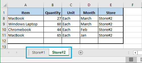
To Create Pivot Table from Multiple Worksheets, let us consider the case of Sales Data from two stores (Store#1 and Store#2) located on two separate Worksheets.
The task is to use these two separate Worksheets as Source Data for the Pivot Table that we are going to create in this example.
Open the Excel File containing Source Data in multiple worksheets.
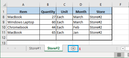
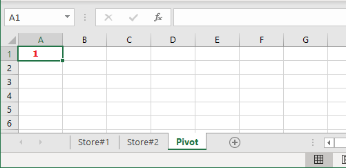
Create a New Worksheet and name it as Pivot. This is where we are going to Create Pivot Table using Source data from multiple worksheets.
Click on any blank cell in the new Worksheet > press and hold ALT+D keys and hit the P key twice to fire up the PivotTable Wizard.
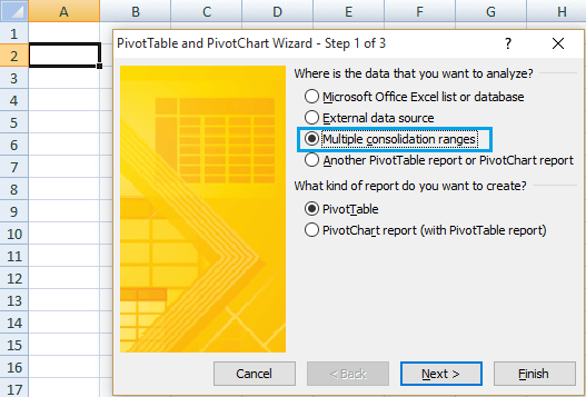
On PivotTable and PivotChart Wizard, select Multiple Consolidation ranges option and click on the Next button
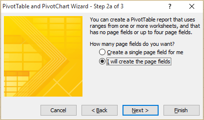
On the next screen, select I will create the page fields option and click Next.
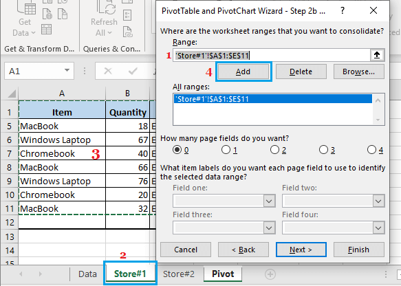
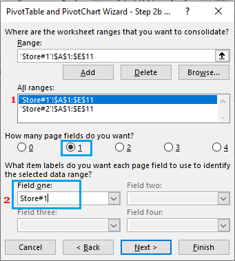
On the next screen, click in the Range Field > click on Store#1 worksheet > select Data Range in this worksheet and click on the Add button.
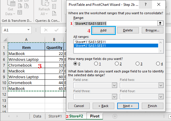
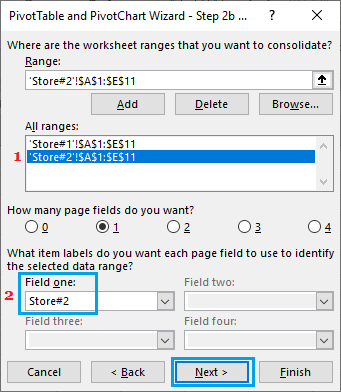
Next, click in the Range Field again > click on Store#2 worksheet > select Data Range in this worksheet and click on the Add button.
- Next, select the first data range in ‘All Ranges’ section and type a Name for this Data Range in ‘Field’ section.
Note: Type a descriptive Name for Data Range, so as to makes it easy for you to identify the Data Range on the pivot table. Similarly, select the second data range in ‘All Ranges’ section > type a Name for this Data Range in ‘Field’ section and click on the Next button.
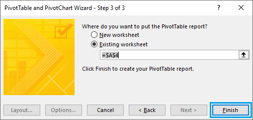
- On the next screen, click on Finish to generate a Pivot Table using Data from multiple worksheets.
Once the Pivot Table is generated, the next step is to modify and format the Pivot Table to suit your reporting requirements.
2. Modify Pivot Table
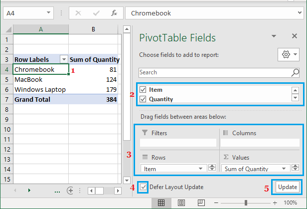
In most cases, the default raw Pivot Table as generated by Excel needs to be modified and formatted to suit reporting requirements. To Modify the Pivot Table click anywhere within the Pivot Table and you will immediately see Pivot Table Field list appearing.
Pivot Table Field list allows you to modify the Pivot Table by dragging the Field List items. If you are New to Pivot Tables, you need to play around with Pivot Table Field List to see what happens when you drag field list items.
3. Format Pivot Table
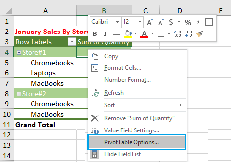
In order to Format the Pivot Table, you will have to open Pivot Table Options.
Right-click on the Pivot table and click on PivotTable Options in the drop-down menu.
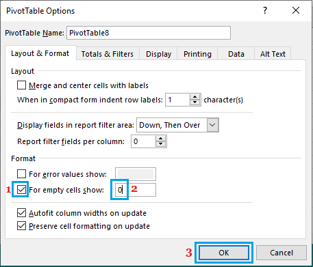
On PivotTable options screen, you will see multiple tabs and various options within each tab to Format the Pivot Table.
Just go ahead and explore all the formatting options as available in different tabs of the Pivot Table Options screen.
How to Create Two Pivot Tables in Single WorkSheet How to Change Pivot Table Data Source and Range How to Fix Empty Cells and Error Values in Pivot Table